Algorithms / Signal Processing — June 2024 completed

FFT_FROM_SCRATCH

A from-scratch Python implementation of the Fast Fourier Transform using the Cooley-Tukey divide-and-conquer algorithm, with performance benchmarking against SciPy's optimized implementation to verify O(n log n) complexity.

Github

The Problem

The Fourier Transform (a mathematical operation that decomposes a signal into the frequencies that make it up) is one of the most useful tools in signal processing. The problem is that the naive discrete version of it, the DFT (Discrete Fourier Transform), requires computing an $N \times N$ matrix multiplication to transform a signal of length $N$ . That’s $O(n^2)$ operations.

For anything resembling real audio, that’s unusable. A 4-minute song sampled at 44,100 Hz gives you roughly 10 million samples. Squaring that is about $10^{14}$ operations. No reasonable amount of hardware saves you from that math.

The FFT (Fast Fourier Transform) is an algorithm that computes the exact same result in $O(n \log n)$ time by exploiting a symmetry in the DFT’s twiddle factors (the complex exponential weights applied at each frequency step). The Cooley-Tukey algorithm, the most common variant, does this by recursively splitting the input into its even- and odd-indexed samples, transforming each half independently, then combining the results using a butterfly operation.

DFT ComplexityO(n²)naive baseline

FFT ComplexityO(n log n)Cooley-Tukey

Largest Input400Ksamples benchmarked

Algorithm

The key insight is the butterfly recurrence. After splitting into even and odd halves and recursively transforming each, the full transform can be assembled in $O(n)$ additional work:

$y_j = y_e[j] + \omega^j \cdot y_o[j]$

$y_{j+n/2} = y_e[j] - \omega^j \cdot y_o[j]$

where $\omega = e^{2\pi i/n}$ is the twiddle factor (a complex root of unity that rotates a point in the complex plane, used here to weight frequency components) and $j$ runs from $0$ to $n/2$ . The minus sign in the second line comes from the symmetry property: $\omega^{j+n/2} = -\omega^j$ . That symmetry is what makes the whole thing work. Instead of computing the full DFT from scratch at every level, you’re reusing the results from both halves and just combining them. The recursion bottoms out at $n=1$ , where the transform of a single sample is just itself.

Why this matters: Each recursion level does $O(n)$ butterfly work, and there are $\log_2(n)$ levels (since you halve the input at each step). That’s where $O(n \log n)$ comes from. The DFT does $O(n)$ work per output frequency bin times $n$ bins, giving $O(n^2)$ . The FFT avoids recomputing shared sub-results by making the recursion explicit.

Implementation Notes

Phase 0

Understanding the DFT

Started by implementing a naive DFT using the full matrix formulation to make the $O(n^2)$ cost concrete. The DFT computes each output frequency bin as a dot product of the input signal against a row of the twiddle factor matrix. Writing it this way makes the quadratic cost obvious: $N$ output bins, each requiring $N$ multiplications.

Phase 1

Recursive FFT

Implemented the Cooley-Tukey radix-2 DIT (Decimation-In-Time) FFT recursively in Python. The implementation splits the input into even and odd indexed samples, recursively calls itself on each half, and combines them using the butterfly recurrence. Input length must be a power of two for this variant, which is a standard constraint satisfied by zero-padding in practice.

Phase 2

Signal Decomposition Demo

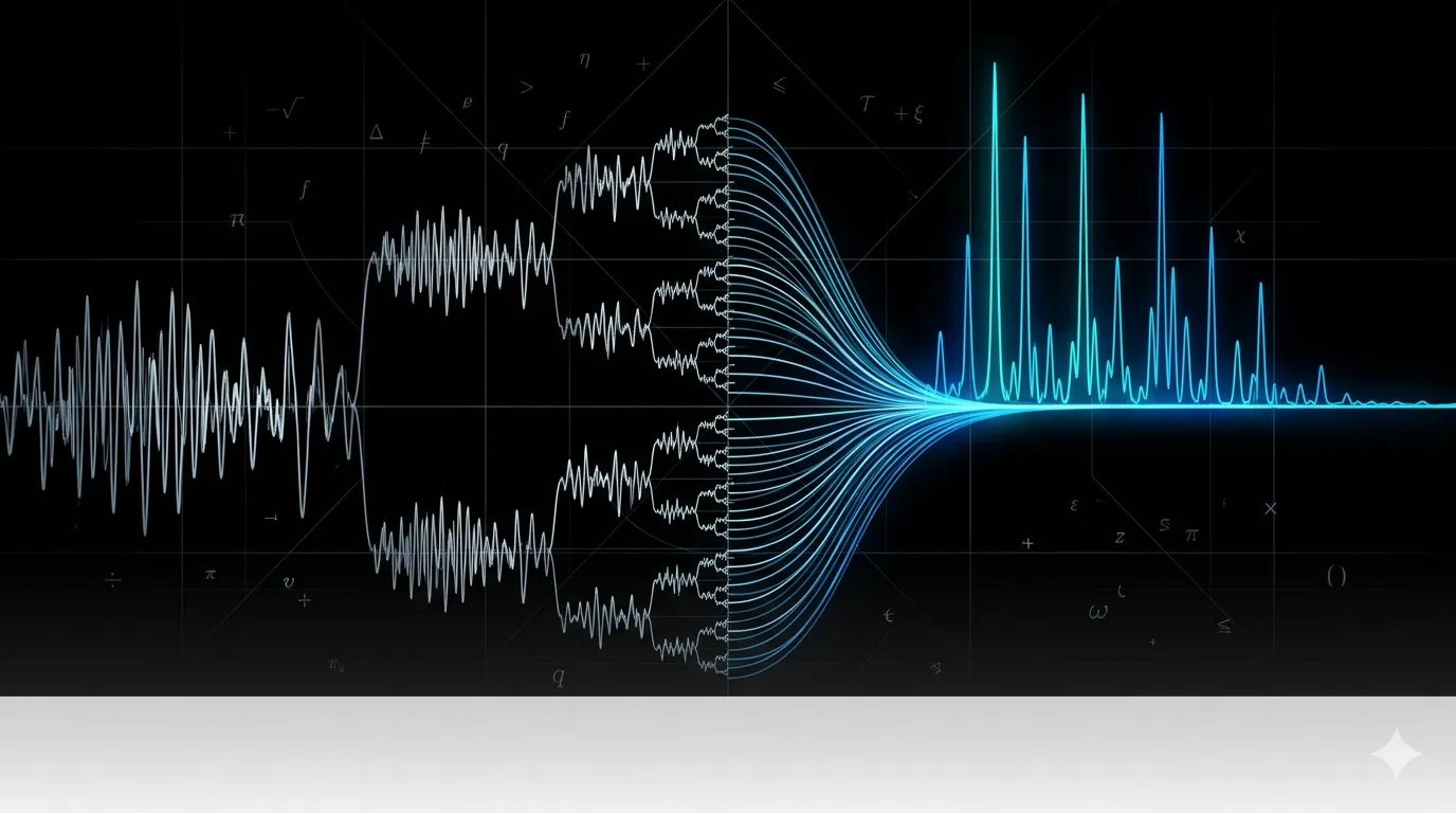
Verified correctness by constructing a composite signal made of two sine waves at known frequencies, running the FFT, and confirming the output peaks matched the input frequencies. The output’s magnitude spectrum shows exactly the two component frequencies, which is the primary practical use of FFT: identifying what frequencies make up an unknown signal.

Phase 3

Benchmarking

Benchmarked the custom implementation against SciPy’s FFT across input sizes from 50,000 to 400,000 samples, running 5 trials per size and averaging. SciPy’s implementation is orders of magnitude faster because it wraps FFTPACK, a Fortran library with vectorized operations and hardware-level optimizations. The custom implementation matches the expected $O(n \log n)$ growth curve in shape but not in absolute speed, which was the expected result: the goal was understanding the algorithm, not competing with a production library.

Key Technical Decisions

Why Python and not a lower-level language? The goal was understanding the algorithm structure, not performance. Python lets you write the recursion clearly and test it quickly without worrying about memory management. The performance gap vs SciPy is a feature here, not a problem. It makes the point: algorithmic complexity matters, but constant factors matter too. SciPy’s FFT is fast not because it uses a fundamentally different algorithm, but because it runs the same algorithm on optimized Fortran routines.

Why benchmark against SciPy instead of a naive DFT? SciPy’s implementation is the real-world baseline worth understanding. A DFT comparison would show the complexity improvement but not calibrate it against anything useful. Comparing against SciPy shows both the complexity match (same asymptotic shape) and the constant factor gap (pure Python overhead vs compiled Fortran), which tells a more complete story.

Lessons Learned

The toughest part was making sure the butterfly recurrence was actually correct before running any benchmarks. The correct output at each recursion level is easy to verify with a 2-element input by hand, but it’s easy to get sign conventions and index arithmetic wrong in the general case. Testing against NumPy’s FFT output on small known inputs before scaling up caught a sign error early.

The other thing worth noting: seeing the output spectrum of a composite signal and recognizing the exact frequencies going in is genuinely satisfying in a way that just reading the math isn’t. The algorithm makes abstract sense on paper; watching it correctly identify that a signal is composed of a 3 Hz and 9 Hz component makes it concrete.